main01.py
Gloals
- compute total cross section in \(ep\) reaction
- generate MC events (inclusive electrons)
Code
First we include some headers
import sys,os
sys.path.append(os.path.dirname( os.path.dirname(os.path.abspath(__file__) ) ) )
import numpy as np
from theory.tools import save, load
from theory.mceg  import MCEG

#--matplotlib
import matplotlib
matplotlib.rcParams['text.latex.preamble']=[r"\usepackage{amsmath}"]
matplotlib.rc('text',usetex=True)
import pylab  as py
from matplotlib.lines import Line2D
from matplotlib.colors import LogNorm
wdir='.main01'
sys.path.append(os.path.dirname( os.path.dirname(os.path.abspath(__file__) ) ) )
will add paths to be able to load the theory module. wdir is where we store
the results.
Next we set physical parameters of the reaction
rs   = 140.7
lum  = '10:fb-1'
sign = 1  #--electron=1 positron=-1
Select lhapdf tables and flavor flags for structure functions
tabname='JAM4EIC'
iset,iF2,iFL,iF3=0,90001,90002,90003
Define a user defined cuts
def veto00(x,y,Q2,W2):
    if   W2 < 10          : return 0
    elif Q2 < 1           : return 0
    else                  : return 1

fname,veto='mceg00',veto00
Create a dictionary with all the parameters
data={}
data['wdir']    =  wdir
data['tabname'] =  tabname
data['iset']    =  iset
data['iF2']     =  iF2
data['iFL']     =  iFL
data['iF3']     =  iF3
data['sign']    =  sign
data['rs']      =  rs
data['fname']   =  fname
data['veto']    =  veto
Build the event generator
mceg=MCEG(data)
mceg.buil_mceg()
The generator will be saved inside wdir.
Next will generate events and store the results
data=mceg.gen_events(ntot)
save(data,'%s/data.po'%wdir)
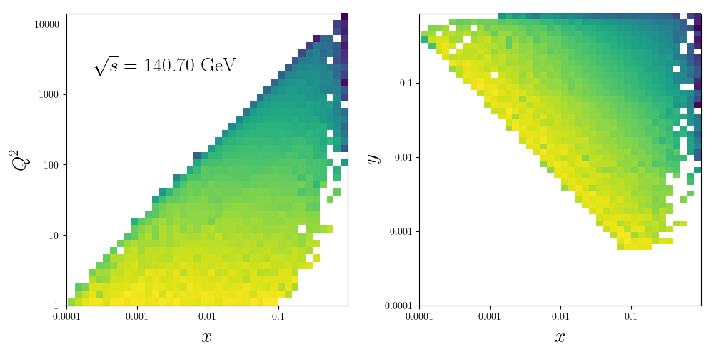
We can now plot the histogram of events
data=load('%s/data.po'%wdir)
X  = data['X']
Y  = data['Y']
Q2 = data['Q2']
W  = data['W']

nrows,ncols=1,2
fig = py.figure(figsize=(ncols*5,nrows*5))

ax=py.subplot(nrows,ncols,1)
ax.hist2d(np.log(X),np.log(Q2),weights=W, bins=40, norm=LogNorm())
ax.set_xticks(np.log([1e-4,1e-3,1e-2,1e-1]))
ax.set_xticklabels([r'$0.0001$',r'$0.001$',r'$0.01$',r'$0.1$'])
ax.set_yticks(np.log([1,10,100,1000,10000]))
ax.set_yticklabels([r'$1$',r'$10$',r'$100$',r'$1000$',r'$10000$'])
ax.set_ylabel(r'$Q^2$',size=20)
ax.set_xlabel(r'$x$',size=20)
ax.text(0.1,0.8,r'$\sqrt{s}=%0.2f{\rm~GeV}$'%rs,transform=ax.transAxes,size=20)


ax=py.subplot(nrows,ncols,2)
ax.hist2d(np.log(X),np.log(Y),weights=W, bins=40, norm=LogNorm())
ax.set_xticks(np.log([1e-4,1e-3,1e-2,1e-1]))
ax.set_xticklabels([r'$0.0001$',r'$0.001$',r'$0.01$',r'$0.1$'])
ax.set_yticks(np.log([1e-4,1e-3,1e-2,1e-1]))
ax.set_yticklabels([r'$0.0001$',r'$0.001$',r'$0.01$',r'$0.1$'])
ax.set_ylabel(r'$y$',size=20)
ax.set_xlabel(r'$x$',size=20)

py.tight_layout()
py.savefig('%s/hist2d.pdf'%wdir)