Tutorial

This documentation explains how to generate the SIDIS cross section:

$$\frac{d\sigma}{dx dQ^2 dz dp_{\rm T}}$$

in units of ${\rm GeV}^{-5}$. Here, $p_{\rm T}$ is the produced hadron’s transverse momentum in the Breit frame and $x,z,Q^2$ are the usual kinematical variables.

Getting started

• Install Anaconda with python2 in your system which you can get for free at https://www.anaconda.com
• Install lhapdf in your system.
• Open up a terminal. Below $ denotes the terminal prompt.
• You will need to make lhapdf reachable from python. For that you need to set the environment variables PYTHONPATH and LD_LIBRARY_PATH. For bash it can be done as

export PATH=<path2lhapdf>/bin:$PATH
export PYTHONPATH=$PYTHONPATH:path2lhapdf/lib/python2.7/site-packages/
export LD_LIBRARY_PATH=<lhapdf>/lib

• Alternatively you can place these lines in your .bashrc file
• Clone the repository from github

git clone git@github.com:JeffersonLab/BigTMD.git

• Go inside the repo directory

cd BigTMD

• Copy the folders lhapdf/dsshpNLO and lhapdf/dsshmNLO inside to

<path2lhapdf>/share/LHAPDF/

• This will allow you to load DSS07 fragmentation functions from lhapdf
• Run the setup script (this takes some time)

./setup.py

• The script sidis.py orchestrates the full NLO calculation for a given kinematic point $x,Q^2,z,q_{\rm T}=p_{\rm T}/z$
• Use driver.py as an example. You can run it simply like

./driver.py

Details

In the above, driver.py calls a function sidis.get_xsec from sidis.py. In turn, sidis.py imports LO.py and the contents of $P_g$ and $P_{pp}$ in the NLO directory. LO.py contains the leading order cross section directly, while $P_g$ and $P_{pp}$ contain all channels and charge configurations for the next-to-leading order cross section. (See citation for explanations of symbols, including $P_g$ and $P_{pp}$.) These functions are of the form

$${\text{ fchn(channel)(charge configuration)}} .$$

The following table summarizes the various incoming and outgoing parton combinations for the virtual and real contributions.

channels index

channel	virtual	real
1	$\gamma^*+g \to(q\to h)+\bar{q}$	$\gamma^*+g \to(q\to h)+\bar{q}+g$
2	$\gamma^*+q \to(q\to h)+g$	$\gamma^*+q \to(q\to h)+g+g$
		$\gamma^*+q \to(q \to h)+q'+\bar{q}'$
3	$\gamma^*+q \to(g\to h)+q$	$\gamma^*+q \to(g \to h)+q+g$
4		$\gamma^*+g \to(g \to h) +q +\bar{q}$
5		$\gamma^*+q \to(\bar{q}\to h)+ q + \bar{q}$
6		$\gamma^*+q\to(q' \to h)+q+\bar{q}$

The channels are organized such that IR singularities of the virtual contribution matches with those from the real contributions. $\gamma^*$ is the virtual photon, $g$ is a gluon, $q$ and $q$ denote different quark flavors, and $\bar{q}$ and $\bar{q}'$ are the antiparticles of $q$ and $q'$ respectively. $f \to h$ means it is the parton of flavor “math:f that hadronizes. For example,

$$\gamma^*+q \to(g \to h)+q+g$$

refers to graphs with 3 unobserved real emissions where a target quark leads to a hadronizing final state gluon and an unobserved quark and gluon. The correspondence between real and virtual graphs is in the sense of Table I of citation.

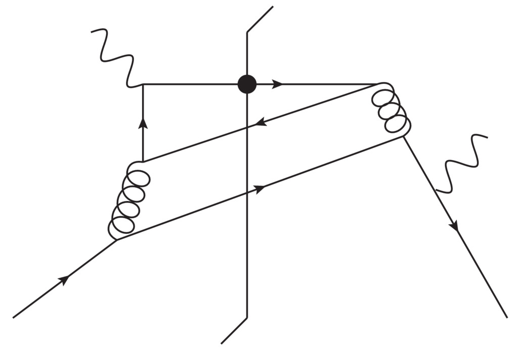
By charge configuration we mean whether the photon couples directly to the charge of a target (anti)quark. A charge configuration $A$ is when the photon couples directly to the quark flavor in the pdf,

configuration $C$ is when it does not,

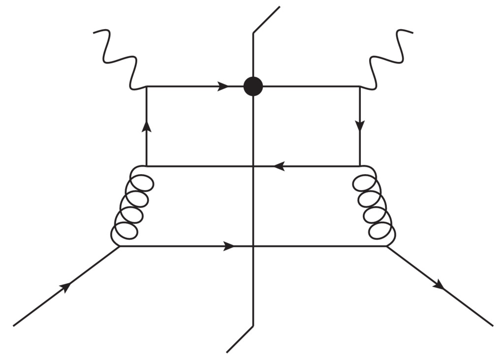
and $B$ is an interference between two such cases. See Fig.``chgcon`` for examples.